What Goes into a Mechanistic Chromatography Model?

Three physical effects, three coupled equations, and a bounded set of experiments to pin them down.

Chromatography rests on three mechanisms, each with its own governing equation: bulk fluid transport through the packed bed, intra-particle diffusion into the pores of the resin beads, and binding at the ligand surface. Each acts on its own timescale, and each leaves a distinct mark on the chromatogram measured at the column outlet.

All three run at once in any column. What differs from one system to the next is their relative magnitude, and therefore how much each one shapes performance.

A mechanistic model writes each of them as a separate term in a single mathematical framework. Every term carries its own parameters, and those parameters correspond to physical effects you can observe and measure. That is what makes the model mechanistic rather than fitted.

It is also what lets you simplify. Start from a comprehensive model containing every mechanism, then strip out the ones that do not matter for the system in front of you.

How Does the Model Work?

Follow a single molecule through the column.

Outside the beads, it travels with the bulk mobile phase, pushed along by the pump. It also spreads out as it goes, because molecular diffusion and the uneven flow paths through the packing broaden the band along the column axis [1].

At the bead surface, convection gives way to diffusion. The molecule crosses a thin stagnant film of liquid, then diffuses inward through the pores of the bead. For a large biomolecule, that inward journey is usually the slowest part of the whole trip [2].

Only then does it bind. Adsorption and desorption at the ligand set how tightly the molecule is held, and therefore what change in conditions is needed to release it again.

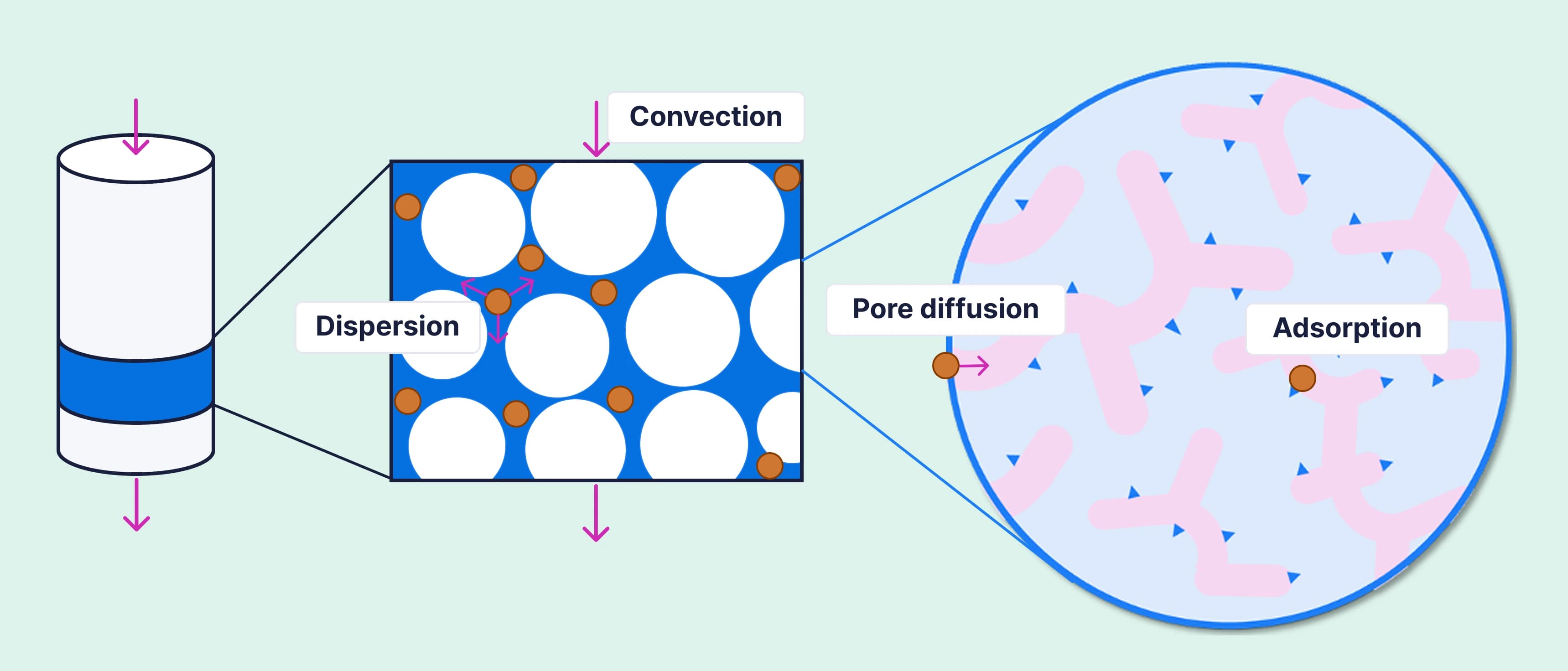
Fig 1. The physical effects inside a chromatography column.

Each effect shows up differently on the chromatogram. Convection sets when the band arrives. Dispersion sets how wide it is. Transport into the beads and binding at the surface decide whether it comes off symmetrical or skewed.

The Governing Equations

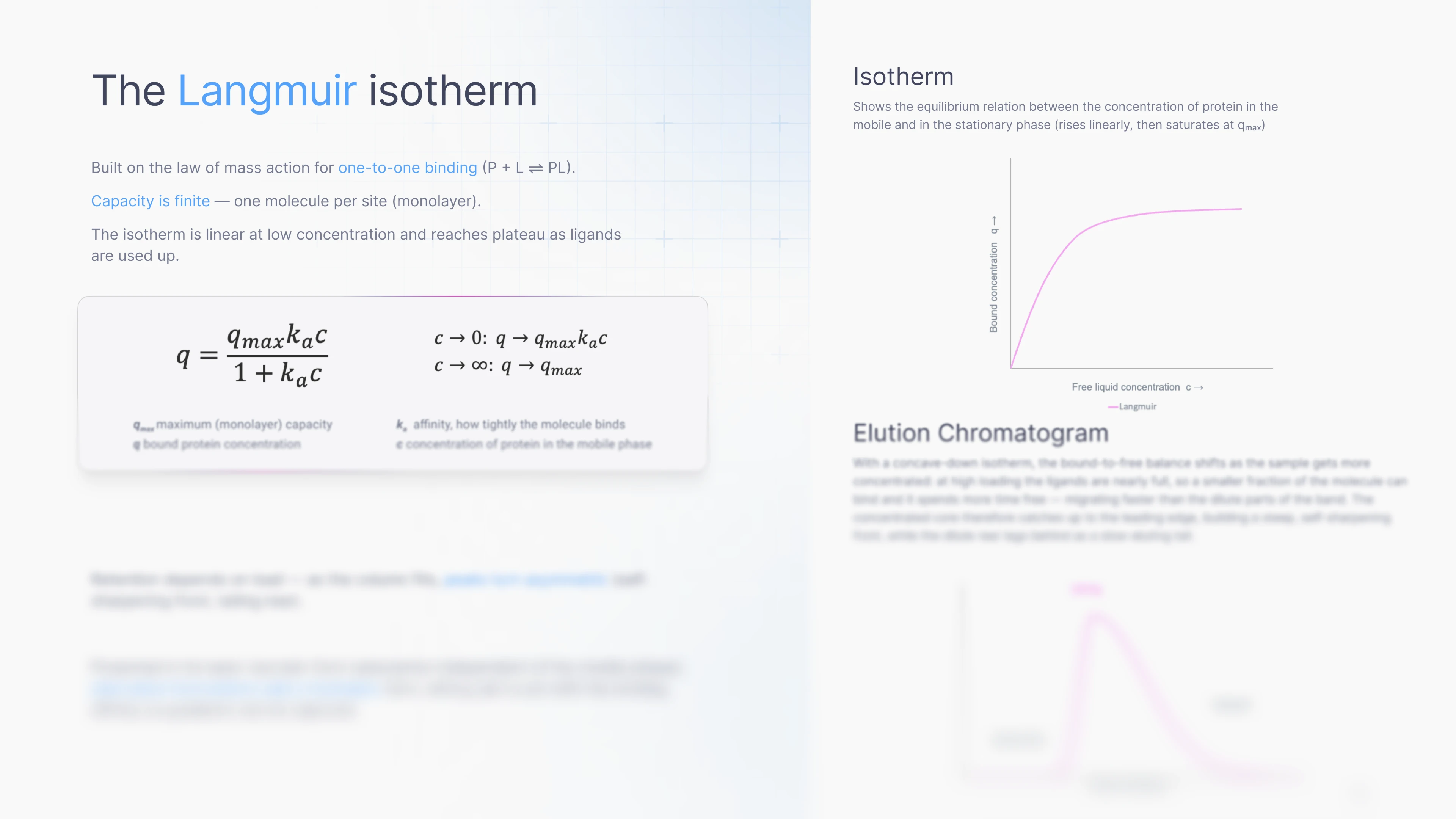
Those three effects are written as equations and solved together as mass balances: one for the liquid between the beads, one for the liquid inside the pores, and an adsorption isotherm for the equilibrium at the surface [1].

The one remaining choice concerns the binding step itself. Where adsorption is fast relative to the flow, it can be treated as local equilibrium and captured by the isotherm alone. Where it lags behind the flow, the rate equations have to be written out explicitly.

The literature offers numerous model variants, each tailored to capture whichever mechanism dominates in a given system [3].

Fig 2. The governing equations of a chromatography model - Langmuir example.

When provided with system-specific parameters and operating conditions, the simulation predicts the outlet concentration profile - matching the chromatogram measured downstream by the detector.

Data Requirements for the Model

Parametrising a mechanistic chromatography model does not require starting from scratch; the required constants fall into three distinct tiers of experimental effort:

Some are known before you start: Column length and diameter, bead radius and dead volume all come from geometry and supplier data.

Some are measured once and then reused: Porosities and the axial dispersion coefficient come from tracer and pulse tests, run once per column and valid for every model built on that column packing afterwards.

The rest are fitted to run data: Thermodynamic and kinetic parameters are estimated by numerical optimisation against measured elution profiles, and the runs feeding that step do not have to be single-component.

Because each parameter imparts a distinct physical signature on the outlet concentration profile, parameter estimation requires relatively few targeted experiments.

Selecting which parameters to fit versus fix requires a structured decision process. Performing a sensitivity analysis identifies which parameters actually drive the elution profile, while parameter correlation matrices reveal which constants can be uniquely identified from the available data. Model-Based Design of Experiments (MBDoE) can then strategically select run conditions that break parameter cross-correlation, achieving full parameter identifiability in significantly fewer runs than conventional factorial screening [5,6].

Four Things You Can Do Once The Model Is Calibrated

• Screen conditions without consuming feed: Different loads, gradient slopes, pH and residence times can all be explored in silico, to identify a process optimised against yield, purity, buffer consumption or resin cycle life.

• Map an operating window rather than a single set point: Sensitivity to salt, pH and load can be quantified across the whole space, which is what proven acceptable ranges and a control strategy are built from.

• Predict at a new scale instead of refitting: Because model terms correspond directly to physical mechanism, scaling up column dimensions or altering flow rates simply requires updating specific coefficients rather than re-evaluating or refitting the model architecture.

• Run it alongside the process as a digital twin: Integrated with inline sensors (e.g., UV, conductivity, pH), the model acts as a real-time digital twin, estimating concentration and purity, flagging operational drift, and offering diagnostic insight into column behaviour [4].

The common thread is that the physics does not change when the process does. Calibrate the model once and it keeps answering questions long after the step itself is fixed.

Need more than an overview?

Translating physics into a mathematical representation of the system requires balancing the dominant mechanisms' effect with your project goals, so you only write as much mathematical complexity as your objectives demand.

We created our guide, Chromatography Modelling: From Physical Phenomena to Predictive Process Models, for downstream scientists, process development engineers, and bioprocess leads evaluating mechanistic modelling for their team. 

The guide breaks down the model selection process to help you:

• Interpret peak behaviour: Connect specific chromatogram shapes back to their underlying physical mechanisms.

• Navigate model tiers: Evaluate the trade-offs between simple lumped models and full transport equations.

• Plan experimental scope: Determine the minimum model detail required before starting laboratory campaigns.

Request the deck.

References

1. G. Guiochon, A. Felinger, D. G. Shirazi, and A. M. Katti, Fundamentals of Preparative and Nonlinear Chromatography, 2nd ed. Amsterdam, The Netherlands: Elsevier Academic Press, 2006. ISBN 978-0-12-370537-2.

2. V. Kumar and A. M. Lenhoff, "Mechanistic modeling of preparative column chromatography for biotherapeutics," Annual Review of Chemical and Biomolecular Engineering, vol. 11, no. 1, pp. 235-255, 2020. doi:10.1146/annurev-chembioeng-102419-125430

3. A. Felinger and G. Guiochon, "Comparison of the kinetic models of linear chromatography," Chromatographia, vol. 60, no. S1, pp. S175-S180, 2004. doi:10.1365/s10337-004-0288-7

4. A. Tiwari, V. S. Masampally, A. Agarwal, and A. S. Rathore, "Digital twin of a continuous chromatography process for mAb purification: Design and model-based control," Biotechnology and Bioengineering, vol. 120, no. 3, pp. 748-766, 2023. doi:10.1002/bit.28307

5. F. Rischawy, D. Saleh, T. Hahn, S. Oelmeier, J. Spitz, and S. Kluters, "Good modeling practice for industrial chromatography: Mechanistic modeling of ion exchange chromatography of a bispecific antibody," Computers & Chemical Engineering, vol. 130, art. 106532, 2019. doi:10.1016/j.compchemeng.2019.106532

6. K. Katsoulas, F. Galvanin, L. Mazzei, M. Besenhard, and E. Sorensen, "Model-based design of experiments for efficient and accurate isotherm model identification in High Performance Liquid Chromatography," Computers & Chemical Engineering, vol. 195, art. 109021, 2025. doi:10.1016/j.compchemeng.2025.109021